Pattern Discovery 2: Null-invariant, Pattern-Fusion, Constaint

패턴 마이닝을 통해 만들어지는 수많은 pattern, rule 이 모두 유용한 것은 아닙니다. 따라서 interestingness measure 을 위해 객관적이거나, 주관적인 평가방법을 이용할 수 있습니다.
(1) Objective interestingness measures
- support, confidence, correlation
(2) Subjective interestingness measures
- Query-based: relevant to a user’s particular request
- Against one’s knowledge-base: unexpected, freshness, timeliness
- Visualization tools: Multi-dimensional, interactive examination
이 방법중, 먼저 객관적인 방법에 대해 좀 더 알아보겠습니다.
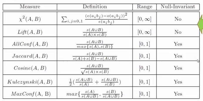
Lift, χ²(Chi-squared)
confidence 는 두 변수가 관련있는지 말해주지만, positive 혹은 negative 관계인지 말해주지 않습니다. 이를 판별하기 위해 lift 를 이용할 수 있죠
Lift(B, C) 는 B 와 C 가 얼마나 관련있는지를 말해줍니다. 수식을 보면 알겠지만
Lift(B, C) = 1이면B와C는 independent> 1이면 positive correlated< 1이면 negative correlated
correlated events 를 판별하는 다른 방법은 χ² 를 이용하는 것입니다.
χ² = 0이면 independentχ² > 1이면 correlated 이며 positive 인지 negative 인지는 expected 값과 비교하면 알 수 있습니다.
![]()
그러나 lift 와 chi-squared 가 항상 좋은 평가지표는 아닙니다. 위 테이블을 보면 Lift(B, C) = 8.44 입니다.
이는 ~B and ~C 부분의 숫자가 B, C 보다 월등히 높아서 그런데, 이런 영역을 null transaction 이라 부릅니다.
B, C 는 같이 일어날 확률이 상당히 낮지만, null transaction 때문에 높은것처럼 보입니다.
Null Invariant Measures
lift 와 chi-squared 는 많은 수의 null transaction 이 있을 때 좋은 평가 지표가 될 수 없습니다.
이를 해결하기 위해 null transaction 에 영향을 받지 않는 null-invaraint measures 를 사람들이 만들어 두었습니다.
null invariance 는 massive transaction data 를 마이닝할때 아주 중요합니다. null transaction 이 아주 많을 수 있기 때문이죠.
그러면 이 많은 measures 중 어떤것이 가장 나을까요? 예제 데이터로 한번 비교해 봅시다. m 은 milk, c 는 coffee 입니다.
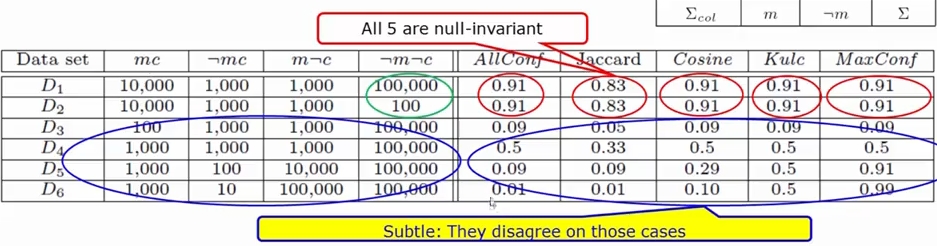
Kulc holds firm and is in balance of both directional implications
여기에 imbalance ratio 라는 개념을 도입할 수 있습니다.
- imbalance ratio: measure the imbalance of two itemsets
AandBin rule implications
Kulc 와 IR 을 이용하면 조금 더 데이터를 자세히 살펴볼 수 있죠.
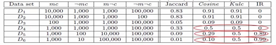
- D4 is neutral, balanced
- D5 is neutral, but imbalanced
- D6 is neutral, but very imbalanced
ID 5 를 보면, Kulc 는 아이템 A, B 가 상당한 연관성이 있지만, imbalance 하므로 0.562 의 값을 돌려주는 것을 볼 수 있습니다.
5. Mining Diverse Patterns
이번 시간에 배울 주제들은 다음과 같습니다.
- Mining Multiple-Level Associations
- Mining Multi-Dimensional Associations
- Mining Quantitative Associations
- Mining Negative Correlations
- Mining Compressed and Redundancy-Aware Patterns
- Mining Long/Colossal Patterns
Multi-Level Associations
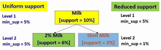
item 은 하위 계층으로 다시 분류될 수 있습니다. 이럴때는 단순히 uniform min support 를 이용하는 것보다, 아래 계층으로 내려갈수록 reduced min support 를 이용하는 편이 더 낫습니다.
그리고 한번의 여러 단계(multi-level) 을 마이닝하기 위해 shared multi-level mining 이란 기법을 이용할 수 있습니다. 이건 뒷부분에서 더 살펴보겠습니다.
multi-level association 마이닝의 문제점은 redundant rules 을 만들 수 있다는 점입니다. 따라서 필터링 기법이 필요합니다. level 1 에서 발견된 룰을, level 2 에서 다시 검사하지 않는것 처럼요
milk -> wheat bread [s=8%, c=70%]2% milk -> wheat breadk [s=2%, c=72%]
아이템에 따라서 customized min support 가 필요한 경우도 있습니다. 우유나 빵은 그렇지 않아도 상관 없지만, diamond, watch 등은 커스터마이징이 꼭 필요합니다. 고가의 아이템이니까요. 이 경우 group-based individualized min-support 를 이용하면 됩니다.
{diamon, watch}: 0.05%; {bread, milk}: 5%;, ...
Multi-Dimensional Associations
multi-dimensional 의 예는
(1) inter-dimension association rules (no repeated pred)
age(X, "18-25") ∩ occupation(X, "student") => buys(X, "coke")
(2) hybrid-dimension association rules (repeated pred)
age(X, "18-25") ∩ buys(X, "popcorn") => buys(X, "coke")
attribute 는 categorical 이거나 quantitative 일 수 있습니다.
Quantitative Associations
numerical attribute (e.g age, salary) 를 마이닝 하기 위해 다양한 method 를 사용할 수 있습니다.
(1) static discretization based on prefefined concept hierarchies. data cube-based aggregation
(2) dynamic discretization based on data distribution
(3) clustering: distance-based association. first one-dimensional clustering, then association
(4) deviation analysis
Negative Correlations
rare pattern 과 negative pattern 은 다릅니다.
(1) Rare patterns
- 아주 낮은 support 지만, 롤렉스 시계를 사는 행위처럼 중요할 수 있습니다
- individualized, group-based min support 를 다양한 아이템 그룹에 설정해서 마이닝합니다.
(2) Negative patterns
- 자동차를 동시에 2개 사는것처럼, 같이 일어나는 경우가 드뭅니다 (unlikely to happen together)
negative pattern 은 어떻게 마이닝할까요? 한가지 방법은 lift 에서 사용했던 support-based definition 을 이용하는 것입니다.
s(A ∪ B) << s(A) X s(B)
이 정의는 작은 transaction dataset 에서는 통하지만, 데이터 크기가 커지면 적용되지 않습니다.
(1) 전체 200개의 트랜잭션에 대해
s(A∪B) = 0.005, s(A) x s(B) = 0.25, s(A∪B) << s(A) X s(B)
(2) 전체 10^5 개의 트랜잭션에 대해
s(A∪B) = 1/10^5, s(A) x s(B) = 1/10^3 X 1/10^3, s(A∪B) >> s(A) X s(B)
이전에 봤었던 null transaction 때문입니다. support-based definition 은 not null-invariant 입니다.
이를 해결하기 위해 Kulczynski measure-based definition 을 이용하면
여기서 ɛ 는 negative pattern threshold 를 의미합니다. 만약 위 수식이 ɛ 보다 작으면 negatively correlated 란 뜻이지요.
Compressed Patterns
때로는 너무 많아 의미가 없는 scattered pattern 때문에 compressed pattern 을 마이닝 할 필요가 있습니다.
compressed pattern 인 closed pattern 과 max pattern 의 정의를 복습해보면
- closed pattern: A pattern
xis closed ifxis frequent, and there exists no super patternY ⊃ Xwith the same support asX - max pattern: A pattern
Xis a max pattern. ifXis frequent and there exists no frequent super-patternY ⊃ X
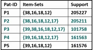
예를 들어 위 그림에서 P1, 2, 3, 4, 5는 모두 closed 고, P3 는 max pattern 입니다. P3 만 남기자니 information loss 가 너무 많고, 다 남기자니 엣지가 없습니다. P2, P3, P4 정도면 적당할 것 같습니다.
이 적당한 정도를 결정하기 위해 pattern distance measure 을 사용할 수 있습니다.
그리고 이 distance 값을 이용해 δ-cluserting 을 합니다.
- δ-clustering: For each pattern
P, find all patterns which can be expressed byPand whose distance to withinδ(δ-cover)
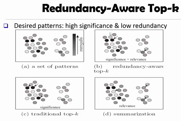
Redundancy-Aware Top-k pattern 이란 기법도 있습니다.
(a) 가 본래 패턴이고, traditional top-k 기법으로는 가장 컴팩트한(진한) 3개의 패턴만 남깁니다. 따라서 우측 클러스터는 버려지죠.
이를 막기 위해 클러스터별로 하나씩 남기는 (d) summarization 을 이용할 수도 있으나, 이건 중요한 것만을 돌려주지 않습니다.
따라서 두 방법을 조합한 (b), 중복을 허용하는 redundancy-aware top-k 를 이용하면 적절한 패턴을 남기고, 나머지는 버릴 수 있습니다.
이를 위해 MMS (Maximal Marginal Significance) 메소드를 사용할 수 있습니다.
Colossal Patterns
long pattern mining 은 소셜 네트워크 분석이나, 바이오인포메틱스, 소프트웨어 엔지니어링등 다양한 분야에서 필요로 합니다. 그러나, 지금까지 우리가 본건 길이가 10 보다 적은 패턴을 마이닝하는 기법들이었습니다.
long pattern 을 분석하기 어려운 이유는 지난시간에 봤듯이 downward closure property 때문입니다. frequent pattern 의 sub-pattern 은 적어도 그만큼은 빈번하기 때문에, 패턴의 길이가 길고 frequent 하다면, 그 수많은 서브패턴을 분석해야 하는 것이지요.
BFS (e.g Apriori), DFS (e.g FPgrowth) 등 무엇을 이용하든 수 많은 패턴을 검색해야 하고, combinatorial explosion 과 마주할 수 밖에 없습니다.
40C20 컴비네이션의 경우 기존에 존재하는 가장 빠른 마이닝 알고리즘들(e.g FP-Close, LCM)도 계산을 완료하지 못하는 경우가 많습니다. 그러나 놀랍게도 pattern-fusion 알고리즘은 1초만에 결과를 돌려줍니다.
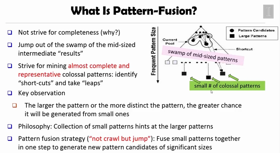
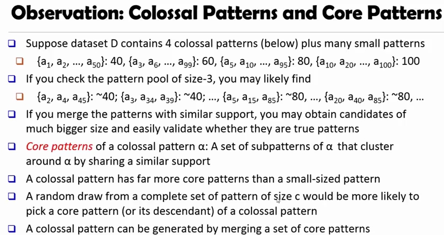
즉, 작은 core pattern 을 모아 colossal pattern 을 만들어 낸다는 것이지요.
- core patterns of a colossal pattern
α: A set of subpatterns ofαthat cluster aroundαby sharing a similar support
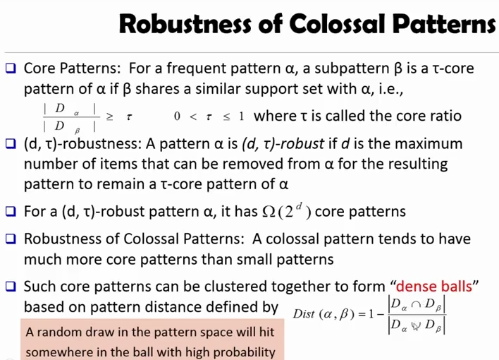
core pattern 에 대한 더 엄밀한 정의는 위와 같습니다.
frequent pattern α 에 대해, sub-pattern 인 β 는 다음을 만족하면 τ-core pattern 입니다.
그리고 패턴 α 에서 d 만큼의 아이템을 제거해도, 여전히 τ-core pattern of α 이면 α 를 (d, τ)-robust 라 부릅니다. 따라서 d 만큼의 아이템이 있거나 없어도, 코어패턴이므로 전체 숫자는 2^d 만큼의 코어패턴을 만들 수 있습니다.
그러므로 colossal pattern 이라면, 정말 많은 수의 core pattern 을 만들 수 있습니다. 그리고 이런 core pattern 은 distance 가 충분히 작으므로 dense ball 형태로 뭉칩니다. 결과적으로 random pattern space 에서 패턴을 뽑으면, dense ball 내의 패턴일 확률이 굉장히 높습니다.
이를 기반으로한 Pattern-Fusion Algorithm 은
- Initialize (creating initial pool):
- Use an existing algorithm to min all frequent patterns up to a small size (e.g 3)
- Iteration (iterative pattern fusion):
- At each iteration,
Kseed patterns are randomly picked from the current pattern pool - For each seed pattern thus picked, we find all the patterns within a bounding ball centered at the seed pattern
- All these patterns found are fused tohether to generate a set of super-patterns
- All the super-patterns thus generated form a new pool for the next iteration
- Termination:
- when the current poll contains no more than
Kpatterns at the beginning of an iteration
6. Constraint-Based Mining
이번시간에 배울 내용은 다음과 같습니다.
- Different Pruning Strategies
- Constrainted Mining with Pattern Anti-Monotonicity
- Constrainted Mining with Pattern Monotonicity
- Constrainted Mining with Data Anti-Monotonicity
- Constrainted Mining with Succinct Constraints
- Constrainted Mining with Convertible Constraints
- Hanlding Multiple Constraints
왜 Constraint-Based Mining 이 필요할까요? 데이터셋에 있는 all 패턴을 autonomously 하게 찾는것은 불가능합니다. 이는 compressed pattern mining 에서 언급했듯이, 너무 많은 패턴이 있기 때문이지요. 특히 데이터셋이 커지면 사용자가 관심 없는 데이터가 기하급수적으로 늘어납니다.
따라서 패턴 마이닝은 사용자가 무엇을 원하는지 data mining query language 나 GUI 를 통해서 직접 명령을 내리는 interactive 한 과정이 되야 합니다.
constraints 를 이용하면 다음과 같은 장점이 있습니다.
- user flexibility: provides constraints on what to be mined
- optimization: explores such constraints for efficient mining
Different Pruning
constraints 에 따라 pruning strategy 달라집니다.
(1) pattern space pruning constraints
- anti-monotonic: if constraint
cis violated, its further mining can be terminated - monotonic: if
cis satisfied, no need to checkcagina - succinct:
ccan be enforced by directly manipulating the data - convertible:
ccan be converted to monotonic or anti-monotonic if items can be propery ordered in processing
(2) data space pruning constraints
- data succinct: data space can be pruned at the initial pattern mining process
- data anti-monotonic: if a transaction
tdoesn’t satisfyc, thentcan be pruned to reduce data processing effort
Anti-Monotonicity
constaint C 는 다음의 경우에 anti-monotone 이라고 말합니다.
- If an itemset
Sviolates constraintC, so does any of its superset - That is, mining on itemset
Scan be terminated
예를 들어서 다음의 제약조건은 anti-monotone 입니다
sum(S.price) <= vrange(S.profit) <= 15support(S) >= k
따라서 Apriori pruning 은 본질적으론 anti-monotonic constaint 에 기반합니다.
반대로 sum(S.price) >= v 는 not anti-monotone 입니다.
Monotonicity
itemset S 가 constaint c 를 만족할때, S 의 superset 도 그러하다면 c 는 monotone 이라 부릅니다. 다음은 모두 monotone 입니다.
sum(S.price) >= vmin(S.price) <= vrange(S.profit) >= 15
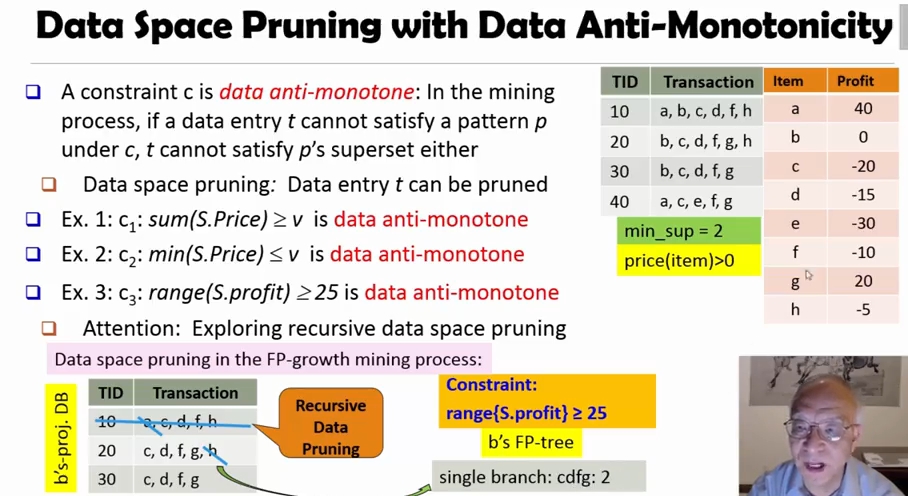
Data Anti-Monotonicity
data anti-monotone 는 transaction 기반으로 pruning 을 진행해 나아갑니다. 정의는 이렇습니다.
- In the mining process, if a data entry
tcannot satisfy a patternpunderc,tcannot satisfyp’s superset either
다음은 모두 data anti-monotone 입니다.
sum(S.price) >= vmin(S.price) <= vrange(S.profit) >= 25
Succinct Constaints
succintness 는 data space 와 pattern space 를 모두 pruning 합니다.
if the constaint
ccan be enforced by directly manipulating the data
(1) To find those patterns without item i
pattern space pruning 처럼 i 을 DB 에서 제거합니다.
(2) To find those patterns containing item i
data space pruning 처럼 i-projected DB 만 마이닝 합니다.
(3) min(S.price) <= v is succinct
price <= v 에서 시작해서, high-price item 을 제거해 나가기 때문에 pattern + data space pruning 입니다.
(4) sum(S.price) >= v is not succinct
itemset S 의 sum 이 점점 크기때문에, 미리 제거할 수 없습니다.
Convertible Constaints
Convert tough constaints into (anti-) monotone by proper ordering of items in transactions
avg(S.profit) > 20 같은 경우는 anti-monotone 도 monotone 도 아닙니다.
- 만약 현재 만족한다고 했을때, 아주 작은
profit*을 가지는 아이템을 추가하면 violation 이고, - 만약 현재 위반한다고 했을때, 아주 큰 값을 추가하면 satisfaction 이기 때문입니다.
이런 constaint 에 대해서도 pruning advantage 를 얻고자 하는것이 바로 convertible constaints 의 목적입니다. 가능하면 anti-monotone 이 더 선호되는데, 이는 monotone 일 경우 검사만 하지 않고, anti-monotone 일 경우 super-pattern 을 날려버릴 수 있기 때문입니다.
- 만약
c: avg(S.profit > 20)에 대해서 - itemset 을 내림차순으로
S: {a, g, f, b, h, d, c, e}정렬하고 avg(ab) = 20,g = 20이면
constaint C 는 anti-monotone 이라 할 수 있습니다. 왜냐하면 패턴 내부가 profit 을 기준으로 내림차순으로 되어서, 어떤 item entry 를 뽑아도 c 를 만족할 수 없기 때문입니다.
아쉽게도 이 방법은 level-wise candidate generation 을 하는 Apriori 알고리즘엔 적용되지 않습니다.
Hanlding Multiple Constaints
다수개의 constaints 를 사용하는것은 좋으나, item ordering 에서 충돌이 생길 수 있습니다. 이럴땐 먼저 하나의 constaint 기준으로 정렬하고, 나머지는 projected databases 를 마이닝할때 하면 좋습니다.
예를 들어 다음 두개의 constaints 가 있을때
c1: avg(S.profit) > 20c2: avg(S.price) < 50
c1 이 더 강력한 pruning power 가 있다고 생각하고, c1 먼저 anti-monotone 으로 변경 한 후, 각 projected-DB 에서 트랜잭션을 오름차순으로 정렬해 c2 를 마이닝에 이용합니다.
Refs
(1) Title image
(2) Pattern Discovery by Jiawei Han
comments powered by Disqus