AI Planning 4: STN, HTN

지금까지 State-Space Planning, Plan-Space Planning 기법을 배웠는데, 이 두 가지는 같은 문제를 푸는 방법이었다. 이제 문제를 조금 변형해, 인간의 사고와 비슷하게 Task 중심으로 분할해서 해결하는 법을 배워보자.
STN
terms 는 constant, variable, object 따위의 것들이고 literals 는 참이거나 거짓이 될 수 있는 proposition 이다.
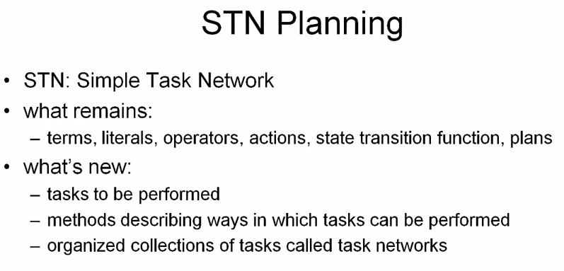
task network 에서 새롭게 도입되는 것은
- task: to be performed
- method: describing ways in which tasks can be performed
- organized collections of tasks: called task networks
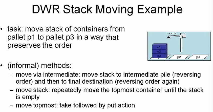
DWR 예제로 보면
Task
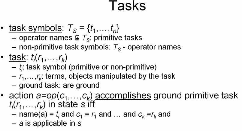
task 는 T_S 처럼 non-primitive 일 수도, t1, ..., tn 처럼 subsete 에 속하는 primitive task 일 수 있다.
task 를 t_i(r1, ..., rk) 라 표기하는데, r 은 task 에 의해 조작되는 object 등의 term 이다.
그리고 슬라이드에 나와 있듯이 ground task 는 variable 이 아니라 action 처럼 constant 를 가져야 하고, action 은 ground primitive task 만 accomplish 할 수 있다.
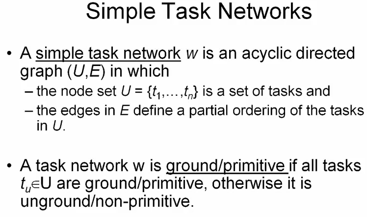
STN 은 acyclic directed graph (U, E) 다. 각 node 는 task 고, edge 는 task 의 partial ordering 을 정의한다. t_i < t_j 처럼
그리고 task network 는 모든 node 가 ground/primitive 일때만 ground/primitive 고, 하나라도 아니라면 unground/non-primitive 다.
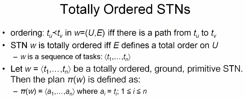
STN w 는 위상 정렬처럼, 모든 edge 가 node 에 대해 순서를 정의할 수 있으면 totally ordered 하다고 말한다. 그러면 w 는 task 의 시퀀스로 나타낼 수 있다. w = <t1, ..., tn>
그리고 w 가 totally ordered, ground, primitive 이면 w 를 위한 plan ㅠ 는
ㅠ(w) = <a1, ..., an> where ai = ti, 1 <= i <= n
DWR 예제로 STN 의 표기법을 알아보자.
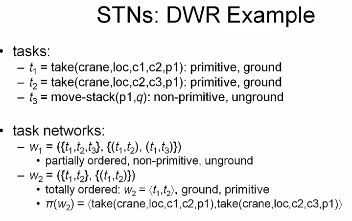
take task 는 똑같은 operator 이름이 있으므로 primitive 고, 변수가 없으므로 ground 다.
move-stack 은 DWR domain 에 정의한 같은 이름의 operator 가 없으므로 non-primitive 이고, 변수가 있으므로 unground 다.
이 3개의 task 를 기반으로 task network 를 구성할 수 있다.
w1 은 (t1, t2), (t1, t3) 고, t2, t3 에 대한 ordering 이 없으므로 partially ordered network 다.
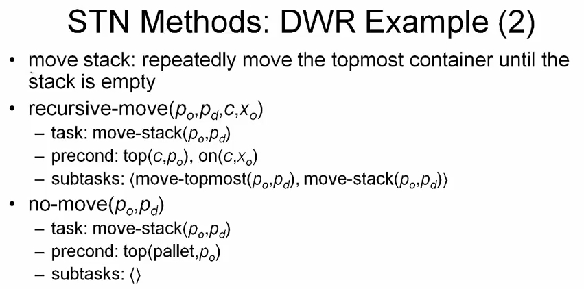
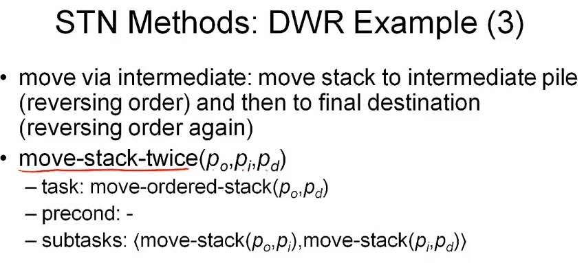
Methods (Refinements)
method: describing ways in which tasks can be performed
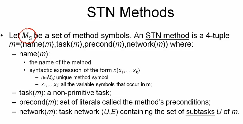
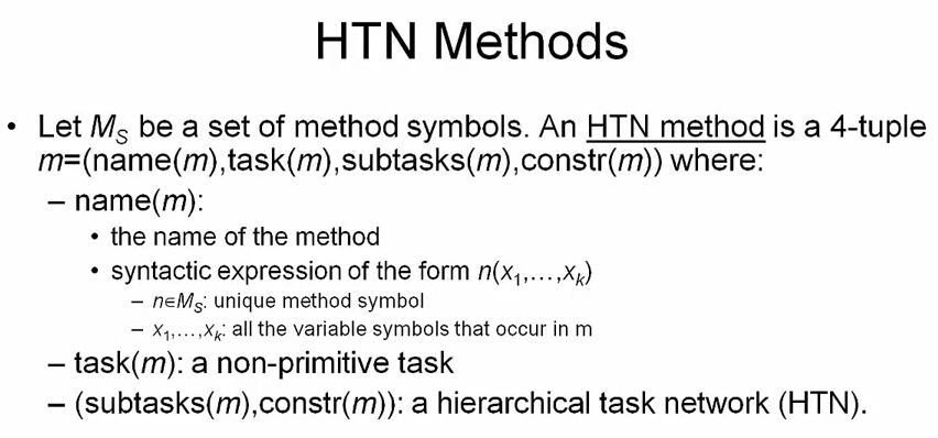
메소드는 name, task, precond network 로 구성되어 있다.
- name(m):
n(x1, ..., xk)의 형태로 unique 한 심볼n과 다뤄지는 variable 인x를 포함한다 - task(m): non-primitive task
- precond(m): set of literals
- network(m): task network
(U, E)containing the set of subtasksUofm
잘 보면 effect 가 없는데, 여기선 goal 을 달성하는 것이 아니라 task 를 수행해야 하기 때문에 effect 는 없고 precond 만 신경쓴다.
그리고 task 는 무엇을 달성해야 하는지를 나타내기 때문에, task 가 같으면 같은 method 가 아니냐고 질문할 수 있으나, network 때문에 다르다. network 는 subtask 를 ordering 한 것으로 어떻게 task 를 수행할지를 나타내기 때문이다.
만약 method 의 network 가 partially ordered 이면 method 도 partially ordered metohd 라 부른다.
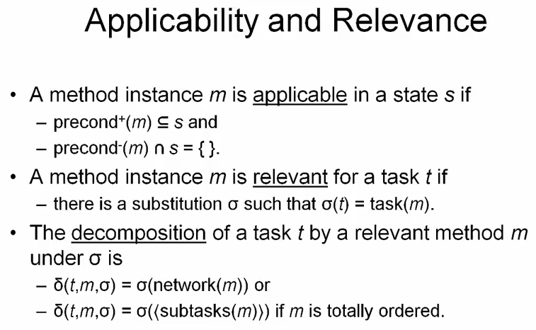
appicability 는 action 과 비슷하다.
만약 substitution σ 에 대해, σ(t) = task(m) 이면 메소드 인스턴스 m 이 태스크 t 와 relevant 하다고 말한다. 왜죠?
무슨 뜻인가 하면, 우리가 달성하려고 하는 t 에 대해 σ(t) 가 메소드의 태스크인 task(m) 과 동일하면, 해당 t 를 위해 메소드 m 을 사용할 수 있다는 뜻이다.
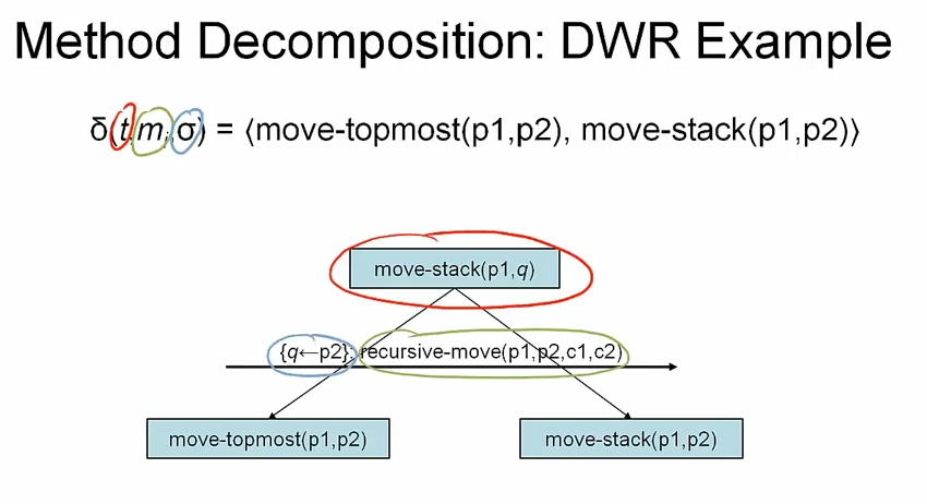
그리고 태스크 t 와 relevant 인 method m 에 대해
δ(t, m, σ) = σ(network(m))또는δ(t, m, σ) = σ(<subtasks(m)>)ifmis totally ordered
로 decomposition 할 수 있다. 그냥 분해인데, 표기법을 저렇게 사용한다고 보면 된다. 당연히 decomposition 되면 subtask 가 되는데, totally ordered 면 subtask 만 돌려주면 되고, 아니라면 network 를 돌려주면 된다는 이야기. DWR 예제로 보자.
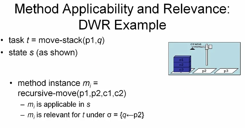
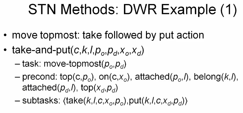
substitution 을 적용했을때task 이름이 같으므로 relevant 하고 precond 를 검사해보면 applicable 하다는 것을 알 수 있다.
Decomposition
method decomposition 을 자세히 살펴보자.
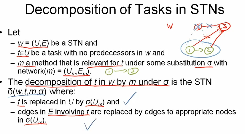
w 를 STN 이라고 하면, U 에 속하는 task t (predecessors 가 없는) 에 대해 relevant 메소드 m 이 있고, substitution σ 와, m 의 network (U_m, E_m) 이 있다. 이 때 decomposition δ(w, t, m, σ) 은
tis replaced inUbyσ(U_m)- edges in
Einvolvingtare replaced by edges to appropriate nodes inσ(U_m)
Domains, Problems and Solution
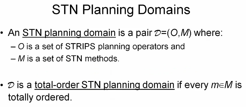
STN planning domain D = (O, M) 이다. O 는 STRIPS planning operators, M 은 STN methods 다. 만약 모든 메소드가 totally ordered 이면 D 도 total-order STN planning domain 이다.
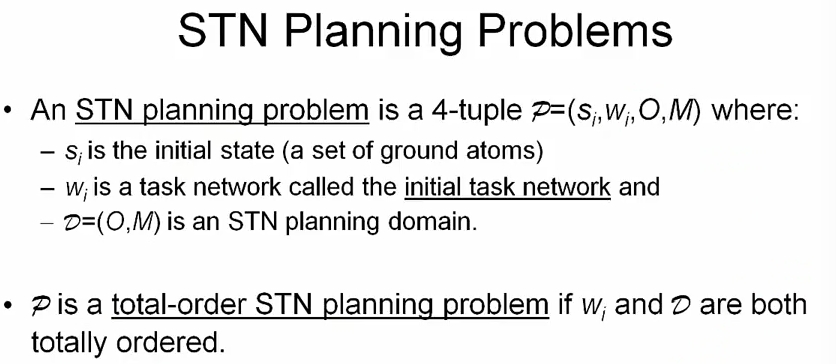
STN planning problem P 는 P = (s_i, w_i, O, M) 으로 구성된다. 잘보면 goal 대신 initial state network 인 w_i 가 있다. w_i 와 D = (O, M) 이 totally ordered 면 P 를 total order STN planning problem 이라 부른다.

(1) w_i 와 plan ㅠ 가 empty 여서 태스크가 없거나
(2) predecessors 가 없는 primitive task t 에 대해, a1 = t 가 s_i 에 applicable 하고, ㅠ = <a2, ..., an> 이 P' = (γ(s_i, a1), w_i - {t}, O, M) 의 솔루션이거나
(3) predecessors 가 없는 non-primitive task t 에 대해 relevant 메소드 m 이 s_i 에 대해 applicable 하고, ㅠ 가 P' = (s_i, δ(w, t, m, σ), O, M) 면 된다.
즉 primitive task 일때는 action 으로 시작하고, 아닐때는 decomposition 한 네트워크에 대해 ㅠ 를 찾으면 된다.
STN Planning
여기서 TFD 는 Total-order Forward Decomposition 의 약자다.
function Ground-TFD(s, <t, ..., tk>, O, M)
  // empty plan, no task
  if k = 0 return <>

  if t1.isPrimitive() thne
    actions = {(a, σ), a = σ(t1) and a applicable in s}

    if actions.isEmpty() then return failure
    (a, σ) = actions.chooseOne()
    plan <- Ground-TFD(γ(s, a), σ(<t2, ..., tk>), O, M)

    if plan = failure then return failure
    else return <a> * plan // add plan

  else
    methods = {(m, σ) | m is relevant for σ(t1) and m is appicable in s}

    if methods.isEmpty then return failure

    (m, σ) = methods.chooseOne()
    // prepend subtasks
    plan <- subtasks(m) * σ(<t2, ..., tk>)

    return Ground-TFD(s, plan, O, M)
DWR 예제를 보면

move-stack 은 non-primitive 이므로 decomposition 하고, 이 과정을 반복하면서 ground, primitive task 를 얻어 action 으로 해결한다.
TFD vs Foward/Backward Search
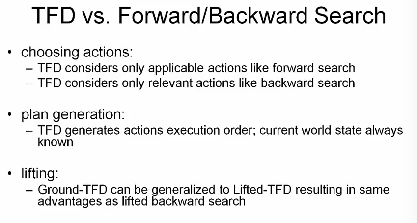
- TFD consider only applicable actions like forward search
- TFD consider only relevant actions like backward search
- TFD generate actions execution order. current world state always known
- Ground-TFD can be generalized to Lifted-TFD resulting in same advantages as lifted backward search
TFD 의 경우 action execution order 를 생성하기 때문에, 현재 어디에 위치해 있는지를 알 수 있다. 이 때문에 goal 까지 더 빠르게 가기 위한 good heuristics 를 적용할 수 있다.
Lifted-TFD 는 variable 을 최대한 유지해, 불필요한 binding 을 막는다.
Partial-order FD 코드도 살펴보자.
function Ground-PFD(s, w, O, M)
  if w.U = {} return <>

  task <- { t ∈ U | t has no predecessors in w.E}.chooseOne()

  if task.isPrimitive() then
    actions = {(a, σ) | a = σ(t1) and a applicable in s}

    if actions.isEmpty() then return failure

    (a, σ) = actions.chooseOne()
    plan <- Ground-PFD(γ(s, a), σ(w-{task}), O, M)

    if plan = failure then return failure
    else return <a> * plan

  else
    methods = {(m, σ) | m is relevant for σ(t1) and m is applicable in s}

    if methods.isEmpty then return failure

    (m, σ) = methods.chooseOne()

    return Gound-PFD(s, δ(w, task, m, σ), O, M)
TFD 와 별 차이가 없다. 초기에 TFD 가 아니므로 인자로 network 인 w 를 받아, task 를 직접 구하는거 이외에는.
HTN Planning
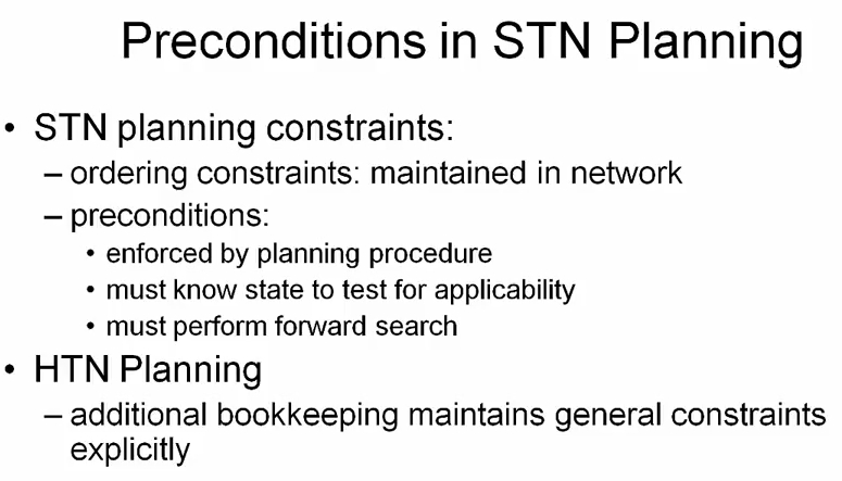
STN planning 에서는 ordering constaints 를 유지해야 하고, applicability 를 테스트하기 위해서 precondition 을 이용했다. 또한 effect 없이 precond 만 이용하므로 반드시 forward search 를 해야 했다.
HTN planning 에서는 ordering constaints 나 precondition 이외에 추가적으로 general constraints 를 유지하여 다른 종류의 constraints 를 조합하는 등 더 유연하게 플래닝할 수 있다.
예를 들어 HTN methods 는 constr(m) 을 포함한다. DWR 예제를 보자.
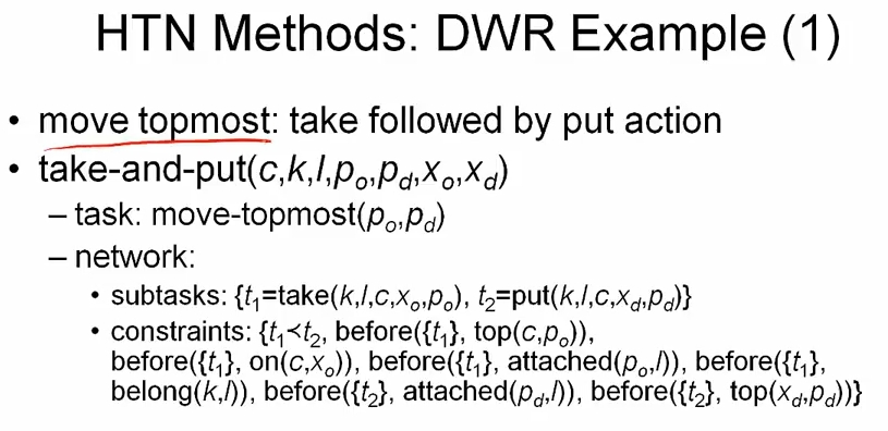
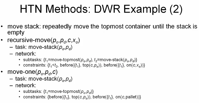
move-one 같은 경우 no-move 대신 이용하는데, 이는 HTN planning 에서는 task 가 없으면 constraints 를 추가할 수 없기 때문이다.
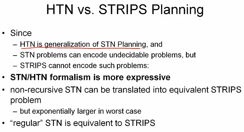
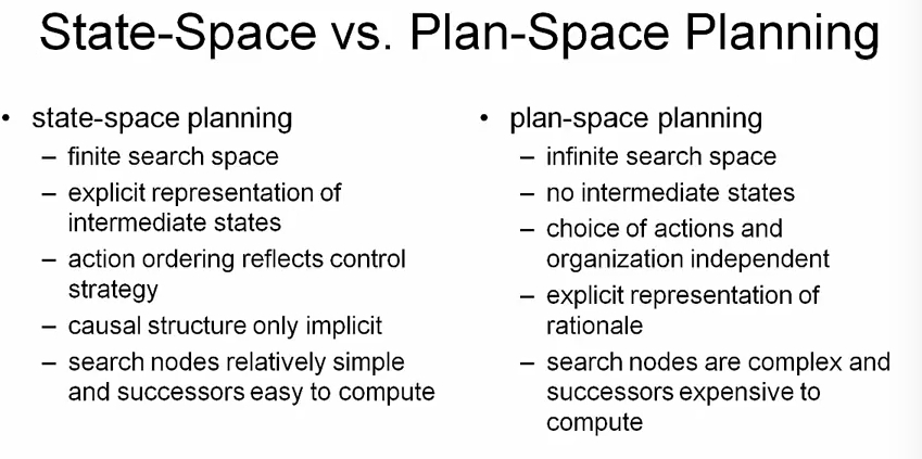
HTN 은 STN 의 더 유연한 버전이고, STN 은 undecidable 한 문제를 풀 수 있지만, STRIPS 에서는 불가능하다. STRIPS 에서는 유한한 오브젝트, 아톰 등으로 구성된 유한한 상태 공간을 탐색하기 때문이다. 반대로 STN 이 background 를 더 필요로 하지만, 더 expressie 함을 알 수 있다.
그렇다고 STRIPS 가 후지다는 것이 아니라, 서로 다른 종류의 문제를 풀 수 있는 두개의 방법이라 보면 된다.
참고로 non-recursive STN 은 STRIPS 로 번역될 수 있다고 한다. 그리고 regular STN 은 STRIPS 와 동일하다고 하는데, regular 란 뜻은 recursive call 이 그리 많지 않은 것을 의미한다.
SIPE-2 HTN Planner
Youtube: SIPE-2 HTN Planner by David Wilkins
Refs
(1) Artificial Integelligence Planning, by Dr.Gerhard Wickler, Prof. Austin Tate
(2) brain image
comments powered by Disqus