Pattern Discovery 1: Apriori, FP Growth

Patterns represent intrinsic and important properties of datasets. Pattern discovery is uncovering patterns (inherent regularities) from massive data sets
- What products were often purchased together?
- What are the subsequent purchases after buying an iPad?
Support, Confidence
;; item bought

Beer, Nut, Diaper
Beer, Coffee, Diaper
Beer, Diaper, Eggs
Nuts, Eggs, Milk
Nuts, Coffee, Diaper, Eggs, Milk
support s 는 전체 구매 중에서, 해당 아이템이 구매되었을 확률이다. min support 를 50% 로 한다면,
- freq 1-itemset: Beer(60%), Nuts(60%), Diaper(80%), Eggs(60%)
- freq 2-itemset: {Beer, Diaper} (60%)
confidence c 는 X 가 포함되어있을때 Y 까지 구매되었을 조건부 확률이다. c = sup(X ∪ Y) / sup(X)
association rule 은, min support 와 min confidence 를 정해놓고, 그 이상이 되는 rule X -> Y 를 찾는 것이다.
Beer -> Diaper(s:60%, c:100%)Diaper -> Beer(s:60%, c:75%)
Closed Patterns
이렇게 패턴을 구하면, 다수개의 물품이 있는 transaction 에서는 너무 많은 패턴이 생긴다.
;; TDB1

T1: {a1, ..., a50}
T2: {a1, ..., a100}
min supoort 를 1 이라 하면 1-itemset, 2-itemset, .. 100-itemset 처럼 2^100 - 1 개의 sub pattern 이 생긴다.
이 문제를 해결하기 위해 lossless compression 인 closed pattern 이란 개념을 도입해 보자.
closed pattern: A pattern(itemset)
Xis closed ifXis frequent, and there exists no super patternY ⊃ X, with the same support asX
위와 똑같은 TDB 에 대해 closed pattern 을 구하면
P1: "{a1, ..., a50}: 2" , P2: "{a1, ..., a100}: 1"
closed pattern 대신 max pattern 을 이용할 수 있다.
max pattern: A pattern
Xis a max-pattern ifXis frequent and there exists no frequent super-patternY ⊃ X
정의를 보면 support 값을 신경쓰지 않는다. 위와 같은 TDB 에 대해 max-pattern 을 찾으면
P: "{a1, ..., a100}: 1
당연히 lossy compression 이다.
Downard Closure Property
Apriori property 라 부르기도 하는데, 핵심은 이렇다.
{beer, diaper, nuts} 가 frequent 하면 subitem 인 {beer diaper} 는 적어도 그 만큼은 frequent 해야한다는 것이다.
Apriori: Any subset of a frequent itemset must be frequent
따라서 S 의 어떤 subset 도 infrequent 하면 S 가 frequent 할 일이 없으므로, 가지치기 할 수 있다는 것이다.
Apriori pruning principle: if there is any itemset which is infreqent, its superset should not even be generated
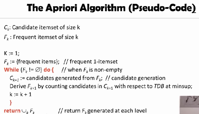
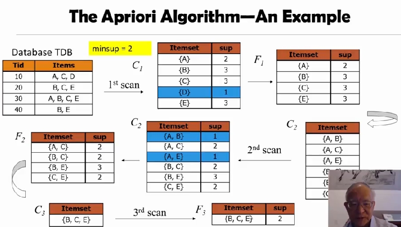
The Apriori Algorithm
level-wise, candidate generation and test
initially, scan DB once to get frequent 1-itemset

repeat
  generate length-(k+1) candidate itemsets from length-k frequent itemsets
  test the candidates against DB to find frequent (k+1) itemset
  Set k := k + 1

until no frequent or candidate set can be generated
apirori 알고리즘이 나온 이래로, 성능을 개선하기 위한 많은 기법들이 발표됬다.
(1) Reduce passes of transaction database scans
- partitioning
- dynamic itemset counting
(2) Shrink the number of candidates
- Hashing
- Pruning by support lower bounding
- Sampling
(3) Exploring special data structures
- Tree projection
- H-miner
- Hypercube decomposition
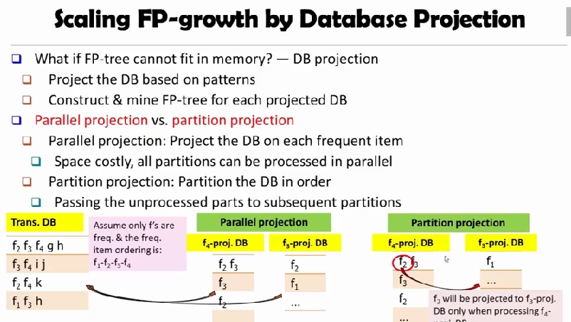
Partitioning
Theorem: Any itemset that is potentially frequent in TDB must be frequent in at least one of the partitions of TDB
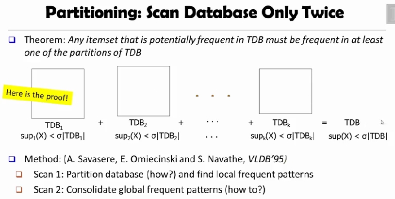
어느 local TDB 에서도 frequent 하지 않으면 global TDB 에서도 frequent 하지 않기 때문에, global 에서 frequent 하려면 적어도 partitioning 된 local TDB 중 하나에서는 frequent 해야 한다.
따라서 scan 1 에서 partitining 하고 local pattern 을 찾고, scan 2 에서 global frequent pattern 을 구하면 된다. 딱 2번만 TDB 에 접근한다.
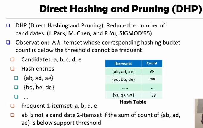
Direct Hashing and Pruning
DHP 는 candidates 의 수를 줄이기 위해 사용하는 기법이다.
observation: A
k-itemset whose corresponding hashing bucket count is below the threshold cannot be frequent
기본적인 아이디어는 item 이 frequent 하다면, hashing bucket 에 들어갔을때 그 count 값이 threshold 보다 높아야 한다는 것이다.
Vertical Data Format
ECLAT (Equivalence Class Transformation) is a depth first search algorithm using set intersection
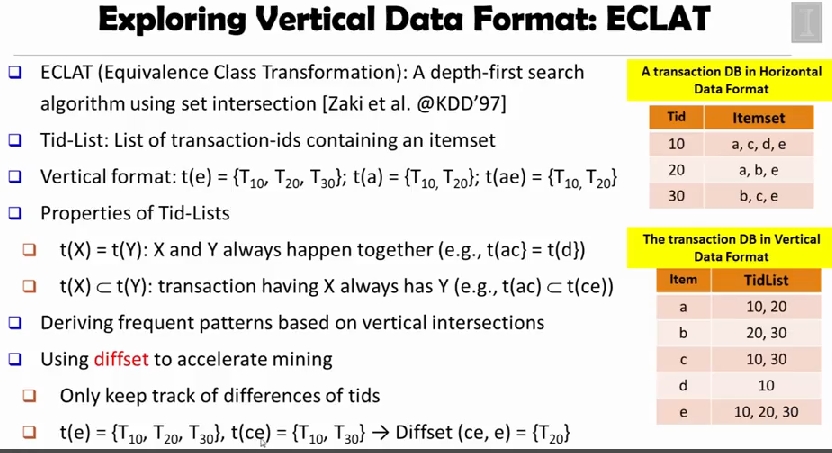
ECLAT 은 item 기준으로 접근하는 방법이다. t(X) = t(Y) 이면 X 와 Y 가 언제나 같이 일어나고, t(X) ⊂ t(Y) 이면 X 가 있을땐 언제나 Y 가 있다.
diffset 연산을 이용하면 공간을 많이 아낄 수 있다. intersection 은 교집합이므로, 공통부분과 그렇지 않은 부분이 생기는데, 다른 부분만 보관하는 것이다.
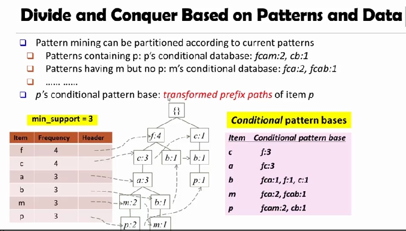
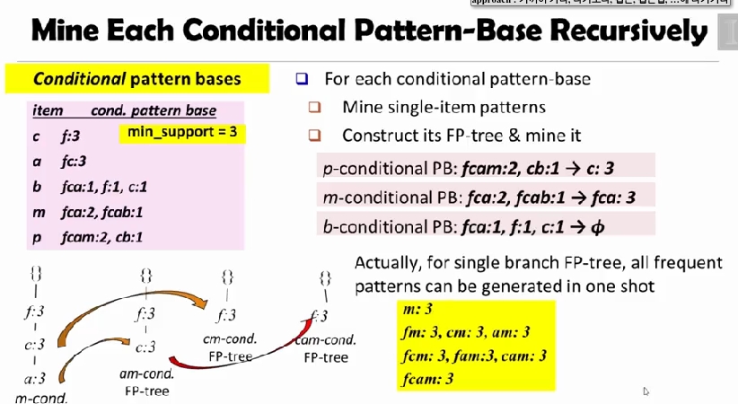
FP Growth
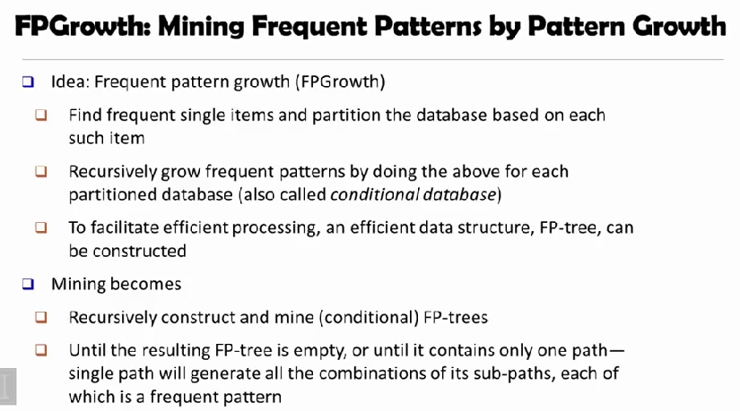
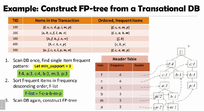
FP-tree 를 만들고, 이를 이용해 conditinal pattern bases 를 구한다.
Mining Closed Pattern
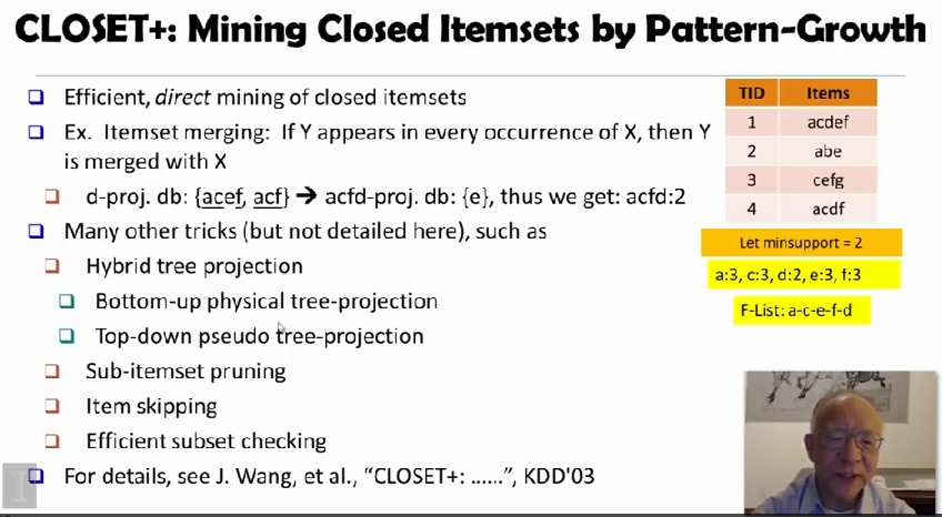
closed pattern 에 대해 쓸 수 있는 다양한 기법이 있다. itemset merging 도 그중 하나인데,
d-proj. db 인 {acef, acf} 를
acfd-proj. db 인 {e} 로 바꾸어, {acfd:2} 를 얻을 수 있다.
이외에도 위 그림에 나온 많은 테크닉들이 있다.
Refs
(1) Title image
(2) Pattern Discovery, Coursera
comments powered by Disqus