Algorithm: Spanning Tree, Shortest Paths
Is a graph bipartite?
그래프가 bipartite 인가 하는 문제는, 그래프의 노드를 이렇게 두 그룹으로 나눌 수 있느냐 하는 문제다.


알고리즘이 얼마나 어려운가는 이렇게 나눠볼 수 있겠는데
- Any programmer could do it
- Typical diligen algorithms student could do it
- Hire an expert
- Intractable
- No one knows
- Impossile
biparting 문제는 DFS-based solution 을 이용할 수 있으므로, 난이도 2정도에 해당한다 볼 수 있겠다.
생각해 볼 수 있는 응용은, 질병의 전파 경로를 그래프로 그리고 biparting 이 가능한지 보는 것이다.
Find a cycle
이것도 난이도 (2) 정도. 마찬가지로 simple DFS-based solution 을 이용하자.
잘 알려진 응용으로, euler tour 가 있다. 각 edge 를 단 한번씩만 방문하는 cycle 이 있는지를 검사하는 문제다. 여기서 시작점과 끝 점이 같으면 euler circuit 이고, 다르면 euler path 라 부른다.
여기에 의하면 그래프에 오일러 회로가 존재하려면
(1) 연결된 그래프여야 하고
(2) 모든 꼭지점의 차수가 짝수여야 한다.
반면 오일러 경로라면, 연결그래프에서 정확히 두 개의 꼭지점만 홀수 차수여야 한다.
각 node 를 정확히 한번씩만 지나는 cycle 을 traveling salesman problem, TSP 혹은 hamiltonian path problem 이라 부른다.
오일러 순회와 경로처럼 시작점과 끝점이 같은지, 아닌지에 따라 구분할 수 있다. hamiltonian cycle 은 전형적인 NP-complete problem 으로 알려져있다. 난이도로 구분하자면 (4) intractable 정도 되시겠다.
Graph Isomorphism Problem
Are two graphs identical except for vertex names?
그래프의 형태가 같은지 묻는 문제다. 예를 들어 다음의 두 그래프는 같은 형태다.

(http://www.biodatamining.org/)
두 그래프의 노드를 n! 으로 배열해 가면서 같은지 비교하는 단순한 방법은 그래프가 커지면 기하 급수적으로 성능이 느려진다. 더 나은 알고리즘이 있는지 연구자들이 노력하고 있지만, 아직 모른다. 난이도는 (5) No one knows
Graphs Planarity
그래프를 crossing edge 가 없는 그래프로 그릴 수 있느냐 하는 문제다.
평면 그래프(planar graph)는 평면 상에 그래프를 그렸을 때, 두 변이 꼭지점 이외에 만나지 않도록 그릴 수 있는 그래프를 의미한다.
이건 난이도 (3) Hier an expert 문제다. DFS 기반의 linear time 알고리즘이 1970년대에 발표되었다.
Minimum Spanning Trees
undirected, positive edge weights 그래프에서
(1) connected, acyclic (tree)
(2) includes all of the vertices (spanning)
인 서브 그래프를 spanning tree 라 부른다.
minimum spanning tree 는 여기서 min weight 를 갖는 spanning tree 를 찾는 문제다.
Applications
- dithering
- cluster analysis
- max bottleneck paths
- network design
등에 활용할 수 있다.
MST: Greedy Algorithm
간단한 설명을 위해서 그래프가 연결되어있고 weight 가 모두 다르다 하자. 그럼 MST 는 하나만 존재할 것이다.
먼저 cut, crossing edge 용어 정리를 하면
Cut: A cut is a graph is a partition of its vertices into two (nonempty) sets
Crossing edge: A crossing edge connects a vertex in one set with a vertex in the other
그러면, 이런 cut property 가 존재한다.
Given any cut, the crossing edge of min weight is in the MST
증명은 min-weight crossing edge e 가 MST 내에 없다고 하자. MST 는 연결되야 하므로 다른 crossing edge f 가 대신 사용될 것이다.
(1) 다른 crossing edge f 가 없으면 connected 가 아니므로 MST 가 아니다.
(2) 만약 f 가 있어서 f 를 대신 사용하는 MST 에 e 를 추가하면 사이클이 생긴다. 이 때 f 를 제거하면 weight 가 더 짧다. 따라서 f 가 포함되면 MST 가 아니다.
따라서 min-weight crossing edge 가 MST 내에 존재한다. 이 사실을 이용하면 MST 를 찾는 greedy algorithm 을 만들 수 있다.
- Start with all edges colored gray
- Find cut with no black corssing edges;
   color its min-weight edge black
- Repeat until V - 1 edges are colored black
즉 어떤 cut 에 대해서 min-weight crossing edge 가 MST 에 포함되므로, 이미 찾은 MST edge 를 포함하지 않는 cut 을 찾아, min-weight crossing edge 을 추가해 나가면 된다.
Correcteness
(1) Any edge colored black is in the MST (vis cut property)
(2) Fewer than V - 1 black edges => cut with no black crossing edges
모든 MST 는 V - 1 개의 edge 로 구성된다. 따라서 V - 1 개의 black edge, 즉 MST 의 원소를 찾아내면 된다.
Edge-Weighted Graph API
public class Edge implements Comparable<Edge> {
  Edge(int v, int w, double weight)
  int either()
  int other(int v)
  int compareTo(Edge that)
  ...
}

// allow self-loops and parallel edges
public class EdgeWeightedGraph {
  EdgeWeightedGraph(int V) // V vertices
  void addEdge(Edge e)
  Iterable<Edge> adj(int v) // edges incident to v
  Iterable<Edge> edges() // all edges
  Int V() // # of vertices
  int E() // # of edges
}

public class MST {
  MST(EdgeWeigtedGraph G)
  Iterable<Edge> edges()
  double totalWeight()
}
Removing assumptions
- What if edge weights are not all distinct?
Greedy MST algorithm still correct if equal weights are present. (our correctness proof fails, but that can be fixed)
- What if graph is not connected?
Compute MS forest = MST of each components
Kruskal’s Algorithm
- Sort edges in ascending order of weight.
- Add next edge to tree T
  unless doing so would create a cycle
  (until V - 1 edges added)
kruskal’s algorithm 은 greedy MST 의 일종이라 볼 수 있다.
선택된 edge e = v <-> w 라 하고 이것을 crossing edge (cut 이라 볼 수 있다), 하면
black edge 간 no cycle 인 e 를 선택한 것이므로 v <-> w 사이엔 black crossing edge 가 없다.
게다가 선택하는 crossing edge 는 가장 작은 weight 를 가진다. 이 전에 이미 더 작은 weight 의 edge 를 모두 선택했기 때문이다.
따라서 크루스칼 알고리즘은 greedy MST 의 일종이다.
Cycle Check
어떻게 Cycle check 를 할까? 한 가지 방법은 edge e = v - w 에 대해 v - w 가 연결되어있는지 DFS 를 돌리면 된다. 그러면 O(V) 로 사이클을 검사할 수 있다.
단순히 연결되어있는지만 검사하는 것이므로 union find 를 쓰면 O(log* V) 로도 가능하다. Union-find 를 참고하자.
Kruskal MST Implementation
EdgeWeightedGraph G;
int V = G.V()
UF uf = new UF(V);

Queue<Edge> mst = new Queue<Edge>();
MinPQ<Edge> pq = new MinQP<Edge>();

for (Edge e : G.edges())
  pq.enqueue(e);

while (!pq.isEmpty() && mst.size() < V - 1) {
  Edge e = pq.dequeue();
  int v = e.either();
  int w = e.other(v);

  if (!uf.connected(v, w)) {
    uf.union(v, w);
    mst.enqueue(e);
  }
}
running time 은 E log E 다.
- build
pq:1 * E - dequeue:
E * log E - union:
V * log* V - connected:
E * log* V
Prim’s Algorithm
- start with vertex 0 and greedily grow tree T
- add to T the min weight edge with exactly one endpoint in T
- repate until V - 1 edge
Correctness
마찬가지로 prim’s algorithm 도 greedy MST 의 일종이다.
방문한 노드와 방문하지 않은 노드를 cut 해 거기서 min-weight edge 를 선택한다. 따라서 cut 자체가 방문하지 않은 노드와 방문한 노드 두 집합을 만드므로 crossing edge 중에는 black edge 가 없다.
Prim MST Implementation
lazy implementation 으로 현재 선택할 수 있는 edge 를 weight 기준으로 priority queue 에 유지하는 방법이 있다.
queue 에 있는 edge e = (v, w) 를 꺼낸 뒤
(1) v, w 둘 다 이미 방문했으면 패스하고,
(2) v 혹은 w 둘 중 하나만 방문했을 경우에만 w or v 의 edge 를 추가하고, w or w 를 방문 처리 한다.
// lazy Prim MST

boolean[] marked // MST vertices
Queue<Edge> mst = new Queue<Edge>();
MinPQ<Edge> pq = new MinPQ<Edge>();
WeightedGraph G;

visit(G, 0);

while (!pq.isEmpty()) {
  Edge e = pq.dequeue();
  int v = e.either();
  int w = e.other(v);

  if (marked[v] && marked[w]) continue;

  mst.enqueue(e);

  // add v or w
  if (!marked[v]) visit(G, v);
  if (!marked[w]) visit(G, w);
}

void visit(int v) {
  marked[v] = true;
  for (Edge g : G.adj(v)) {
    if (!marked[e.other(v)]) pq.insert(e);
  }
}
running time 은 O(E log E) 다.
좀 더 나은 알고리즘은 MST 에 edge e = (v, w) 를 추가할때, 이미 방문한 w 와 방문하지 않은 v 에 대해
v 에서 갈 수 있는 모든 edge e = (v, x) 을 생각해 보면,
(1) x 가 이미 방문한 vertex 면 패스
(2) queue 에 (k, x) 가 없으면 추가 (k 는 이미 방문한 vertex)
(3) x 까지의 거리가, e = (v, x) 가 더 짧으면 업데이트 (decreaseKey operation)
여기서 decreaseKey 연산을 빠르게 구현하기 위해 indexed priority queue 를 이용할 수 있다.
void decreaseKey(int i, Key key)
전체 러닝타임은
VinsertVdelete minEdecrease key
인데, Priority Queue 구현하는데 어떤 자료구조를 사용하느냐에 따라 각 연산의 시간이 달라진다.
(1) Array implementation optimal for dnse graph
O(V^2)
(2) Binary heap much faser for sparse graphs
O(E log V)
(3) 4-way heap worth the trouble in performance-critical situations
O(E log_(1/V) V)
(4) Fibonacchi heap best in theor, but not worth implementing
O(E + V log V)
MST Context
linear time MST 알고리즘이 있을까? 1995년에 linear time randomized MST 가 발견 되었지만 deterministic 알고리즘은 여전히 연구중이다.
Shortest Paths API
public class Directed Edge {

  DirectedEdge(int v, int w, deouble weight)
  int from()
  int to()
  double weight()
}

// allow self-loop, parallel
public class EdgeWeightedDigraph {

  EdgeWeightedDigraph(int V)
  void addEdge(DirectedEdge e)
  Iterable<DirectedEdge> adj(int v)
  int V() // # of vertices
}

// shortest path
public class SP {

  SP(EdgeWeightedDigraph G, int s)
  double distTo(int v)
  Iterable <DirectedEdge> pathTo(int v)
}
Shortest Path Properties
directed, weighted graph 에서 shortest path tree, SPT 가 존재하는데, 이는 cycle 이면 shortest 가 될 수 없기 때문이다.
위에서 본 pathTo 함수는 이렇게 구현할 수 있다.
// edgeTo[v] is last edge on shortest path from s to v
public Iterable<DirectedEdge> pathTo(int v) {
  Stack<DirectedEdge> path = new Stack<DirectedEdge>();
  for (DirectedEdge e = edgeTo(v); e != null; e = edgeTo(e.from())
    path.push(e);

  return path;
}
Edge relaxation
relax edge e = v -> w,
distTo[v]is length of shortest known path fromstovdistTo[w]is length of shortest known path fromstowedgeTo[w]is last edge on shortest known path fromstow
여기서 만약 e = v -> w 가 w 로의 더 짧은 거리라면, distTo[w] 와 edgeTo[w] 를 업데이트하면 된다.


(http://www.csupomona.edu/~ftang)
void relax(DirectedEdge e) {
  int v = e.from();
  int w = e.to();

  if (distTo(w) > distTo(v) + e.weight()) {
    distTo[w] = distTo[v] + e.weight();
    edgeTo[w] = e;
  }
}
Shortest-paths optimality conditions
Let
Gbe an edge-weighted digraph, thendistTo[]are the shortest path distance from s iff:
distTo[s]= 0- For each vertex
v,distTo[v]is the length of some path fromstov - For each edge
e = v -> w,distTo[w] <= distTo[v] + e.weight()
necessary condition
만약 어떤 e = v -> w에 대해 distTo[w] > distTo[v] + e.weight() 이면, e 를 이용한 w 까지의 거리가 distTo[w] 보다 더 짧다. 그러면 distTo[w] 는 shortest path 가 아니다.
sufficient condition
- Suppose
s = v0 -> v1, ... -> vk = wis a shortest path fromstov
그러면
distTo[v1] <= distTo[v0] + e1.weight();
...
distTo[vk] <= distTo[v_k-1] + ek.weight();

// e_i is, i th edge on shortest path from s to w
이제 distTo[v] = 0 이라 하면
distTo[w] <= e1.weight + ..., + ek.weight()
이 때 우변이 shortest path 위에 있는 edge 의 weight 값이므로, distTo[w] 는 w 까지의 shortest path 다.
(여기서는 필요충분조건 p <=> q 를 증명하기 위해 p -> q, q -> p 를 증명했다.)
Generic Shortest-paths Algorithm
initialize distTo[s] = 0 and distTo[v] = infinity for all other vertices

Repeat until optimality conditions are satisfied,
  Relax any edge
어떤 edge 를 고를까 하는 문제로 발전할 수 있다.
(1) Dijkstra’s algorithm: non-negative weights
(2) Topological sort: no directed cycles
(3) Bllman-Ford algorithm: no negative cycles
Dijkstra’s Algorithm
- Consider vertices in increasing order of dinstance from s
  (non-tree vertex with the lowest distTo[] value)

- Add vertex to tree and relax all edges pointing from that vertex
Correctness
Dijkstra’s algorithm computes a SPT in any edge-weighted digraph with non-negative weights
모든 e = v -> w 는 단 한번씩만 relaxed 되기 때문에 알고리즘은 언젠간 종료된다. (v 가 T 에 추가되었을 때)
그리고 이 과정에서 distTo[w] <= distTo[v] + e.weight() 가 유지된다. 왜냐하면 distTo[w] 는 줄어들기만 하고, weight 가 음수인 edge 가 없기 때문에 distTo[v] 는 변함이 없기 때문이다.
DirectedEdge[] edgeTo;
double[] distTo;
IndexMinPQ<Double> pq;

void DijkstraSP(EdgeWeightedDigraph G, int s) {
  int V = G.V();
  edgeTo = new DirectedEdge[V];
  distTo = new double[V];
  pq = new IndexMinPQ<Double>(V);

  for(int v = 0; v < V; v++) {
    distTo[v] = Double.POSITIVE_INFINITY;
  }

  distTo[s] = 0.0;
  pq.insert(s, 0.0);

  while (!ps.isEmpty()) {
    int v = pq.dequeue();
    for(DirectedEdge e: G.adj(v))
      relax(e);
  }
}

void relax(DirectedEdge e) {
  int v = e.from();
  int w = e.to();

  if (distTo[w] > distTo[v] + e.weight()) {
    distTo[w] = distTo[v] + e.weight();
    edgeTo[w] = e;

    if (pq.contains(w)) pq.decreaseKey(w, distTo[w]);
    else pq.insert(w, distTo[w]);
  }
}
프림 알고리즘과 마찬가지로
T(n) = V insert + V delete-min + E decrease key 인데, 이 연산들은 Priority Queue 구현에 따라 다를 수 있다.
undordered array 라면 V^2, binary heap 이라면 E log V
따라서 dense graph 에서는 array 를, sparse graph 라면 binary heap 이 낫다.
Dijkstra and Prim
둘 다 spanning tree 를 만들어 낸다.
- 다익스트라는 directed path 에서 source 에서 가장 가까운 vertex 를 선택한다면,
- 프림 알고리즘은 undirected edge 내 에서 tree 에서 가장 가까운 vertex 를 선택한다.
Edge-Weighted DAGs
cycle 이 없는 그래프는 shortest path 를 찾기 더 쉽다.
toplogical order 순서로 relaxing 해 가면 된다. 어차피 방문 자체는 topological order 로 해야만 모든 vertex 를 방문할 수 있기 때문이다.
이 알고리즘에서 재미난 점은 음수 weight 가 있던 말던 상관이 없다는 것이다.
Topological sort algorithm computes SPT in any edge-weighted DAG in time proprotional to
E + V
다익스트라와 마찬가지로 모든 edge e = v -> w 는 단 한번만 relaxed 되고, 이 과정에서 distTo[w] <= distTo[v] + e.weight() 다.
(1) distTo[w] 는 줄어들기만 하고,
(2) topological order 이기 때문에 한번 방문된 v 에 대해 이후의 vertex 에서 v 로 갈 수 없다. 있다면 cycle 이고 그럼 toplogical order 가 안된다. 따라서 distTo[v] 는 변하지 않는다. 따라서 weight 가 음수든 양수든 상관이 없다.
DirectedEdge[] edgeTo;
double[] distTo;

public AcyclicSP(EdgeWeightedDigraph G, int s) {
  int V = G.V();
  edgeTo = new DirectedEdge[V];
  distTo = new double[V];

  for(int v = 0; v < V; v++) {
    distTo[v] = Double.POSITIVE_INFINITY;
  }

  distTo[s] = 0.0;

  Topological t = new Topological(G);

  for (int v : t.order()) {
    for (DirectedEdge e : G.adj(v)) {
      relax(e);
    }
  }
}
응용으로 seam carving 이 있다. 수직이나 수평으로 shortest path 를 찾아서 제거하면 된다.

(http://rahuldotgarg.appspot.com)
longest path 를 찾는법은 모든 weight 를 negate 하고, 찾고, 다시 결과의 weight 에 마이너스를 붙이면 된다. 이게 가능한 이유는 no cycle 이기 때문에 weight 가 음수든, 양수든 상관이 없기 때문이다.
응용해서 Critical path method, CPM 에 활용할 수 있다.
작업간 의존관계가 있으므로 이를 이용해서 DAG 를 그리면 된다. 각 job 당 start vertex, finish vertex 가 되며, 그 weight 는 duration 으로 하고 한 작업과 다음 작업의 weight 는 0 으로 했을때의 longest path 를 찾으면 된다.
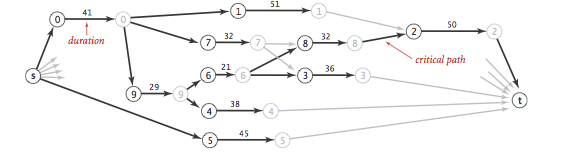
(http://algs4.cs.princeton.edu/44sp/)
Negative Weights
다익스트라 알고리즘은 negative weight 에 대해서 작동하지 않는다. 모든 weight 에 일정 수 n 을 더해 모두 양수로 만들어도 똑같다. 심지어 이 경우는 shortest path 자체가 바뀐다. 따라서 다른 알고리즘이 필요하다.
진도를 빼기 전에 용어를 좀 정의하고 가면
negative cycle 은, directed cycle 내의 모든 weight 를 더했을 때 음수인 경우를 말한다. 이 경우 SPT 는 없다. 이는 쉽게 보일 수 있는데
negative cycle 이 존재하면 한번 이 사이클을 돌면, 전체 값이 음수이므로 어느 경로를 택해도 이전보다 더 짧아진다.
따라서 이 사이클을 돌면 내부 vertex 를 무한정 relaxing 할 수 있다.
Bellman-Ford Algorihm
Bellman-Ford Algorihm 은 negative cycle 이 있는지 검사할 수 있다.
- Initialize
distTo[s] = 0anddistTo[v] = inffor all other vertice - Repeat V times, relax each Edge
for (int i = 0; i < G.V(); i++)
  for(int v = 0; v < G.V(); v++)
    for(DirectedEdge e: G.adj(v)) // pass i
      relax(e);
벨만 포드 알고리즘은 negative cycle 이 없을때 O(E * V) 로 shortest path 를 찾아낸다.
증명은 여기를 참조하도록 하자.
알고리즘을 잘 보면, 한 pass 에서 distTo[v] 가 변하지 않으면 그 이후에도 안 변한다.
If
distTo[v]does not change during passi, no need to relax any edge pointing fromvin passi + 1
따라서 distTo[] 가 변화한 v 의 리스트를 유지해서, 이것 대상으로 relax 하면 성능을 더 개선할 수 있다.
Finding a negative cycle
벨만 포드 알고리즘은 negative cycle 을 찾아내는데 사용할 수도 있다. negative cycle 이 있을 경우 무한히 relax 를 해 내기 때문이다.
따라서 V - 1 까지 진행 한 후 V 번째에서 어느 vertex v 라도 업데이트 된다면, negative 사이클이 있다.
negative cycle 은 arbitrage detection 에 사용할 수 있다.
Shortest Path Cost Summary
(1) Topological Sort: No directed cycles
다익스트보다 더 빠르고, negative weight 도 문제 없다.
- typical:
E + V - worst:
E + V - extra space:
V
(2) Dijkstra(binary heap): No negative weights
거의 linear time 이다.
- typical:
E logV - worst:
E logV - extra space:
V
(3) Bellman Ford: No negative cycles
- typical:
E * V - worst:
E * V - extra space:
V
(4) Bellman Ford(queue): No directed Cycles
- typical:
E + V - worst:
E * V - extra space:
V
SPT 를 정리하면
directed cycle 은 문제를 더 어렵게 만들고, negative weight 도 문제를 더 어렵게 만들고, negative cycles 는 문제를 풀 수 없게 만든다. (내가 배운 한도 내에서는)
References
(1) Algorithms: Part 2 by Robert Sedgewick
(2) Wikipedia: Bipartite Graph
(3) http://www.biodatamining.org/
(4) Wikipedia: 평면그래프
(5) CS241 Lecture Notes: Graph Algorithms
(6) Seam Carving for Content-Aware Image Resizing
(7) Algorithms: Shortest Path
(8) What does bellman ford algorithm
comments powered by Disqus