Intro to Data Science 4
그래프는 네트워크를 표현하는 것 뿐만 아니라, state 를 표현할 수 있다.
- Nodes represent states of system
- Edges represent actions that cause a change of state
그러면 그래프 문제는
- Finding sequence of actions to convert system to desired state

8 puzzle 도 이렇게 그래프 문제로 변환할 수 있다. 그런데, 9! = 362880 의 node 와 노드당 2~4 개의 edge 를 가지고 있으므로 문제의 사이즈가 어마어마하게 커진다. 거의 백만개의 edge 를 가진다.
An Implicit Graph
그래서, 처음부터 모든 state 를 만들기 보다는 초기 상태로부터 action 을 취해가면서 desired state 를 찾는 방식으로 해결하자.
퍼즐의 상태를 문자열로 표현하면
class puzzle(object):
    def __init__(self, order):
        self.label = order

        for i in range(9):
            if order[i] == '0':
                self.spot = i
                return None

    def transition(self, to):
        currentLabel = self.label
        blank = self.spot
        # current slot value which will be filled with blank
        current = str(currentLabel[to])
        nextLabel = ''

        for i in range(9):
            if i == to:
                nextLabel += '0'
            elif i == blank:
                nextLabel += current
            else:
                nextLabel += str(currentLabel[i])

        return puzzle(nextLabel)

    def __str__(self):
        return "{0} {1} {2}\n{3} {4} {5}\n{6} {7} {8}\n".format(self.label[0],
                                                                self.label[1],
                                                                self.label[2],
                                                                self.label[3],
                                                                self.label[4],
                                                                self.label[5],
                                                                self.label[6],
                                                                self.label[7],
                                                                self.label[8])
그리고 각 슬롯의 이동 가능한 방향을 딕셔너리로 만들면
shiftDict = {}
shiftDict[0] = [1, 3]
shiftDict[1] = [0, 2, 4]
shiftDict[2] = [1, 5]
shiftDict[3] = [0, 4, 6]
shiftDict[4] = [1, 3, 5, 7]
shiftDict[5] = [2, 4, 8]
shiftDict[6] = [3, 7]
shiftDict[7] = [4, 6, 8]
shiftDict[8] = [5, 7]
이제 state 를 변경해 나아가면서 그래프를 만들 수 있다 state, 즉 node 를 변경해 나아가면서 그래프를 탐색하는 방법은 2개가 있는데, BFS, DFS 다. 코드는 거의 유사하다. 스택을 쓰냐 큐를 쓰냐의 차이다.
def notInPath(state, path):
    for s in path:
        if s.label == state.label:
            return False

    return True


def BFS(start, end, q=[]):
    initPath = [start]
    q.append(initPath)

    while len(q) != 0:
        currentPath = q.pop(0)
        lastState = currentPath[len(currentPath) - 1]

        if lastState.label == end.label:
            return currentPath

        for s in shifts[lastState.spot]:
            nextState = lastState.transition(s)

            if notInPath(nextState, currentPath):
                nextPath = currentPath + [nextState]
                q.append(nextPath)

    return None


def DFS(start, end, stack=[]):
    initPath = [start]
    stack.insert(0, initPath)

    while len(stack) != 0:
        currentPath = stack.pop(0)
        lastState = currentPath[len(currentPath) - 1]

        if lastState.label == end.label:
            return currentPath

        for s in shifts[lastState.spot]:
            nextState = lastState.transition(s)

            if notInPath(nextState, currentPath):
                nextPath = currentPath + [nextState]
                stack.insert(0, nextPath)

    return None
테스트는
def test():
    goal = puzzle('012345678')
    test1 = puzzle('125638047')
    answer = BFS(test1, goal)

    for state in answer:
        print state
비교해 보면 BFS 가 훨씬 빠르다.
Maximum Cliques
For some problems, finding sugraphs of a graph that are complete can be important
여기서 complete 란 노드가 다른 노드 모두와 연결되어 있다는 뜻이다.
- Finding sets of people in a social network that all know each other
- Finin subjects in an infected population that all have had contact with one another
두 번째 예제는 complete subgraph 를 찾는 것의 중요성을 잘 보여준다.
clique 는 communication networks, gene expression data 등에도 이용할 수 있다.
Brute Force
maximum clique 문제를 brute force 로 풀려면, 가능한 모든 서브 그래프를 찾고, clique 인지 판별하면서 큰 사이즈의 clique 를 유지하면 된다.
모든 서브 그래프를 찾을려면, 지난시간 에 knapsack problem 을 풀 때 이용했던 power set 을 도입하면 된다.
knapsack 문제도 brute force 로 풀기 위해서 가능한 모든 집합을 구했었다. 후에는 search space 를 줄이기 위해 decision tree 를 도입하고, 반복 계산을 피하기 위해 memoization 이용했었다.
clique 문제도 마찬가지로 각 노드를 숫자로 표현할 수 있으므로 n 자리의 이진수를 만들어 power set 을 생성할 수 있다. 지난 시간에 이용했었던 대강의 로직은
count = 2 ** len(nodes)

binStrs = []

for i in range(count):
  binStrs.append(int2bin(i, len(nodes))

powerSet = []

for bs in binStrs:
  subGraph = []

  for i range(len(bs)):
    if bs[i] == '1':
      subGraph.append(nodes[i])

  powerSet.append(subGraph)

return powerSet
이번시간엔 재귀를 이용해서 power set 을 구해보자. 하스켈로 로직을 표현하면,
powerset [] = [[]]
powerset (x:xs) = xs' ++ map (x:) xs'
  where xs' = powerset xs
따라서 파이선 코드는
def powerSet(xs):
    if len(xs) == 0:
        return [[]]

    else:
        # xs = head:tail
        head = xs[0]
        tail = xs[1:]

        prev = powerSet(tail)
        incl = map(lambda sub: sub + [head], prev)
        return prev + incl
이걸 이용해 모든 sub graph 를 만들고, clique 인지 검사하는 함수를 만들면
def powerGraph(graph):
    nodes = []

    for n in graph.nodes:
        nodes.append(n)

    pSet = powerSet(nodes)
    return pSet


def isClique(graph, subGraph):
    for n in subGraph:
        for m in subGraph:
            if not m == n:
                if n not in graph.childrenOf(m):
                    return False

    return True


def maxClique(graph):
    maximum = None
    maxLen = 0
    subGraphs = powerGraph(graph)

    for sub in subGraphs:
        if isClique(graph, sub):
            if len(sub) > maxLen:
                maximum = sub
                maxLen = len(sub)

    return maximum
지난시간에 작성했던 Graph 코드 는 여기로,
테스트 코드는
def testGraph():
    nodes = []
    for name in range(5):
        nodes.append(Node(str(name)))
    g = Graph()
    for n in nodes:
        g.addNode(n)
    g.addEdge(Edge(nodes[0],nodes[1]))
    g.addEdge(Edge(nodes[1],nodes[2]))
    g.addEdge(Edge(nodes[2],nodes[0]))
    g.addEdge(Edge(nodes[2],nodes[4]))
    g.addEdge(Edge(nodes[4],nodes[3]))
    return g


trialGraph = testGraph()
myClique = maxClique(trialGraph)
myClique 를 출력하면, node 가 3개 나와야 한다.
Machine Learning
Automating automation
Computer programs can automatically follow rules.
How do we determine these rules automatically?ML fources on getting computers to program themselves
Let the data do the work.
Automatically generate programs that create useful outputs from data
전통적인 프로그래밍에선 data 와 program 을 넣고 output 을 기대했다면,
machine learning 에서는 data, output 을 넣고 program 을 만든다. 이 프로그램은 다음번에 data 가 들어왔을 때 output 을 만들어 낸다. 다시 말해서 머신러닝은 일종의 generalization 이다.
Supervised
Given a set of feature/label pairs, find a rule that predicts the label associated with a previously unseen input
Unsupervied
Given a set of feature vectors (without labels), group them into “natural clusters”
예를 들어 다음은 supervised learning 이다.
A group of 1000 students are asked for a sample of their handwriting. Researchers make pairs of (handwritten text, typed text). Given a new handwriting sample from a new student, we want to determine what the typed version of the handwriting sample would be.
Clustering
- Low intra-cluster dissimilarity
- High inter-cluster dissimilarity
간단하긴 한데, 연산 비용이 비싸다. k-means 와 hierarchical clustering 을 살펴보자.
Hierarchical Clustering
(1) Start by assigning each item to a cluster, so that if you have N items, you now have N clusters, each containing just one item.
(2) Find the closest (most similar) pair of clusters and merge them into a single cluster, so that now you have one cluster fewer.
(3) Continue the process until all items are clustered into a single cluster of size N
(http://www.alanfielding.co.uk)
Linkage Criteria
in single-linkage clustering (also called the connectedness or minimum method), we consider the distance between one cluster and another cluster to be equal to the shortest distance from any member of one cluster to any member of th other cluster
in complete-linkage clustering (also called the diameter or maximum method), we consider the distance between one cluster and another cluster to be equal to th greatest distance from any member of one cluster to any member of the other cluster
in average-linkage, we consider the distance between one cluster and another cluster to be equal to th average distance from any member of one cluster to any member of the other cluster. A slight variant of this uses the median instead of the mean
single-linkage 클러스터 간 거리를 두 클러스터 사이의 최소 거리로, complete-linkage 는 최대 거리로, average-linkage 는 평균 거리로 본다.
    def singleLinkageDist(self, other):
        """ Returns the float distance between the points that
        are closest to each other, where one point is from
        self and the other point is from other. Uses the
        Euclidean dist between 2 points, defined in Point."""
        minDist = float("inf")
        for p1 in self.points:
            for p2 in other.points:
                dist = p1.distance(p2)
                if dist < minDist:
                    minDist = dist

        return minDist

    def maxLinkageDist(self, other):
        """ Returns the float distance between the points that
        are farthest from each other, where one point is from
        self and the other point is from other. Uses the
        Euclidean dist between 2 points, defined in Point."""
        maxDist = float(0)
        for p1 in self.points:
            for p2 in other.points:
                dist = p1.distance(p2)
                if dist > maxDist:
                    maxDist = dist

        return maxDist

    def averageLinkageDist(self, other):
        """ Returns the float average (mean) distance between all
        pairs of points, where one point is from self and the
        other point is from other. Uses the Euclidean dist
        between 2 points, defined in Point."""
        dists = []
        for p1 in self.points:
            for p2 in other.points:
                dists.append(p2.distance(p1))

        return sum(dists) / float(len(dists))
K-Means Clustering
- Final result can depend upon initial centroids
- Greedy algorihm can find different local optima
- Choosing the wrong
Kcan lead to nonsense
따라서
- Use priori knowledge about application domain
- Try multiple times
hierarchical 과 비교하면
Hierarchical looks at different numbers of clusters From 1 to n
K-means looks at many ways of createing k clusters.
hierarchical 은 좀 느린편이고 deterministic 이다. 반면 K-means 는 비교적 빠르고, stochastic 이다.
아래는 K-means 로 분류하기 어려운 몇 가지 예제들
(https://courses.edx.org/c4x/MITx/6.00.2_2x)
Scaling
odd ratio 는 acutal / expected 값인데, 1에 가까우면 클러스터링이 랜덤에 비해 별로 나을게 없다는 소리다. (좋은 클러스터링이 아니란 뜻)
강의에서 나온 환자 예제는 이 값이 1에 근접하는데, 이는 HR, age 값이 단위가 커서 이 feature 에 영향을 많이 받기 때문이다.
따라서 평균 0, 표준편차 1을 가지도록 모든 feature 를 스케일링 하고 다시 돌리면 odd ratio 0.18, 1.45 의 두 클러스터를 얻을 수 있다. 하나는 heart attack 이 잘 안올 환자, 다른 하나는 위험한 환자.
아래 예제는 스케일링 하면 안되는 경우
The percent concentration of a virus in a random sampling of healthy and unhealthy people.
The angle of refraction of light (degree that light bends) observed when entering water vs. glass vs a diamond.
Statistical Fallacies
세상에는 3 종류의 거짓말이 있다고 한다.
- LIES
- DAMNED LIES
- STATISTICS

(http://en.wikipedia.org/wiki/Anscombe's_quartet)
보면 데이터가 정말 다르게 분포해 있지만, mean, variance, correlation, linear regression 이 동일하다.
흔한 오류 중 하나로, correlation => causation 도 있다.
학교가 문을 여는 시즌에, 독감이 많이 유행한다고 해서 상관 관계가 있다고 단정짓긴 어렵다. 어쩌면 다른 요인이 있을지도 모른다.
non response bias 도 생각해봐야 한다. 예를 들어 전화조사에서, 응답자와 비응답자의 정치 성향이 다를 수도 있다는 것이다.
Data Enhancement
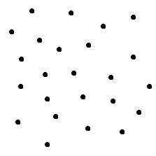
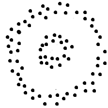
texas sharpshotter fallacy (텍사스 명사수의 오류) 란 것도 있다. 위키 에서 인용하면
The Texas sharpshooter fallacy is an informal fallacy which is committed when differences in data are ignored, but similarities are stressed.
텍사스의 총잡이가 헛간에 총을 마구마구 쏜 후, 밀집한 지역 중심으로 원을 그리면! 그 총잡이는 명사수처럼 보이게 된다는 것에서 유래한 오류다.
바꿔 말하면, 우연도 필연으로 해석한다는 것이다. (존재하지도 않는 패턴을 찾으려고 하는것에 비유하기도 함)
References
(1) MIT 6.00.2 2x in edx
(2) Wikipedia: Huristic Function
(3) http://www.alanfielding.co.uk
(4) Wikipedia - Anscombe’s quartet
comments powered by Disqus