Posted in Algorithm, coursera, reduction, convex hull
Problem Reduction
Comment

앞으로 남은 3챕터에서 배울 내용은
reduction, linear programming, intractability 이다.
따라서 지금까지의 관심에서 좀 벗어나
- from individual problems to problem-solving models
- from linear / quadratic to polynomial / exponential scale
- from details of implementation to conceptual framework
Intro to Reduction
reduction 챕터에서는 다음의 내용을 다룬다.
- design algorithms
- estabilish lower bounds
- classify problems
reduction 의 정의부터 보면
Problem
Xreduces to problemYif you can use an algorithm that solvesYto help solveX
따라서 X 를 푸는데 드는 비용은 reduction 과, Y 를 해결하는 비용의 합이다.
median 을 찾는 문제의 경우, 정렬문제로 변환할 수 있다. 이 때의 비용은 N logN + 1인데, reduction (post or preprocessing) 비용이 1 이다.
중복 원소를 제거하는 문제의 경우 정렬뒤, 인접한 원소간 비교하여 제거하는 문제로 치환할 수 있다. N logN + N 의 비용으로, 이 경우 reduction 비용은 N 이다.
min cut 의 경우 max flow 알고리즘을 이용해서 풀 수 있고, reduction 하는데 DFS 또는 BFS 로 한번 돌려야 하므로, 치환 비용은 V + E 다.
이외에도 다양한 reduction 예제가 있다.
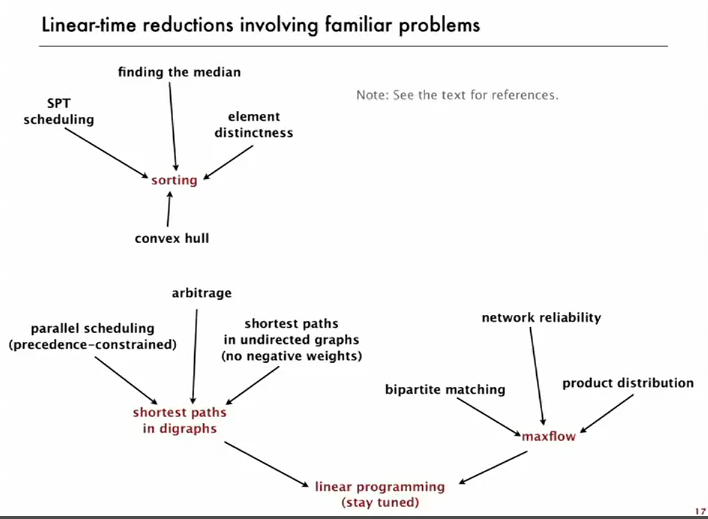
- 3-collinear -> sorting
- CPM -> topological sorting
- arbitrage -> shortest path (벨만포드)
- Burrows-Wheeler transform -> suffix sort
따라서 Y 문제를 풀 수 있을때, X 에 적용 가능한지가 문제가 된다.
Convex hull

(http://cgm.cs.mcgill.ca/~orm)
convex hull 은 sorting 으로 바꿀 수 있다.
convex hull: Given
Npoints in the plane, identify the extream points of the convex hull (in counterclockwise order)sorting: Given
Ndistinct integers, rearrange them in ascending order
reduction 가능한지는 Graham scan algorithm 으로 증명된다. 비용은 N logN + N 으로, reduction 에 N 만큼의 비용이 든다.
Graham Scan
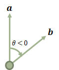
먼저 cross product (외적) 에 대해 잠깐 보고가자. 내적은 스칼라지만, 외적은 또 다른 벡터를 돌려준다. 두 벡터에 대해 수직인 벡터를 돌려주고, 그 크기는 두 벡터로 만들어지는 평행사변형의 넓이다.

외적은 벡터를 돌려주고, 그 방향이 sin 에 기반하기 때문에 두 벡터 a, b 의 외적 a x b 의 값에 따라 a 를 기준으로 b 가 좌측에 있는지, 우측에 있는지 알 수 있다. 위 그림에서 b 가 아래쪽을 향할때 a x b 의 방향이 어디가 될지 생각해 보자.

이제 graham scan 알고리즘을 보면
- choose point
pwith smallest y-coordinate - sort points by polar angle with
pto get simple polygon - consider points in order, and discard those that would create a clockwise turn
polar angle 은

(http://www.yourdictionary.com)
그리고 clockwise turn(시계방향) 인지 아닌지 외적으로 구할 수 있다. 외적값이 음수면 시계방향이다.
따라서 최초의 다각형에서, 선분을 순회하면서 현재 선분과 다음 점을 외적해서 반시계 방향인 점들만 택하면 된다. 그러므로 정렬 + 순회이므로 linear time 이다.
Shortest Path
(non-negative weights) undirected graph 의 최단거리도 directed graph 로 치환해서 풀 수 있다. 각 edge 에 양쪽으로 모두 방향을 추가하면 된다. 러닝타임은 E logV + E, 여기서 E 는 reduction cost 다.
Can still solve shortest paths problem in undirected graphs (if no negative cycles), but need omre sophistcated techniques
Linear-time reductions
Establishing Lower Bounds
comparison-sorting 알고리즘의 lower bound 는 n log n 임을 이전 강의에서 봤었다. Lower bound for sorting 참조
일반적으로 어떤 문제의 lower bound 를 알긴 상당히 난해한데, reduction 을 이용해서 어떤 문제가 sorting 처럼 이미 lower bound 가 알려진 문제로 변경할 수 있다면 lower bound 를 알 수 있다. (reduction cost 가 그리 크지 않다고 한다면)
Linear-time reductions
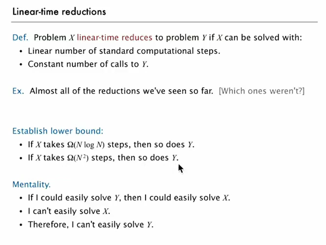
Problem
Xlinear-time reduces to problemYifXcan be solved with
- Linear number of standard computational steps
- Constant number of calls to
Y
따라서 문제 X 를 Y 로 linear-time reduction 이 가능하다면 같은 lower bound 를 적용할 수 있다. X 가 k 시간이 걸린다면, Y 도 그러하다는 것이다.
그리고 Y 를 더 빨리 풀 수 있는 기법이 개발되면 X 에도 적용 가능하다는 뜻이다.
Lower bound for convex hull
Proposition: in quadratic decision tree model (allows linear or quadratic tests), any algorithms for sorting
Nintegers requiresΩ(N logN)stepsProposition: sorting linear-time reduces to convex hull. So if I can solve convex hull efficiently, I can sort efficiently
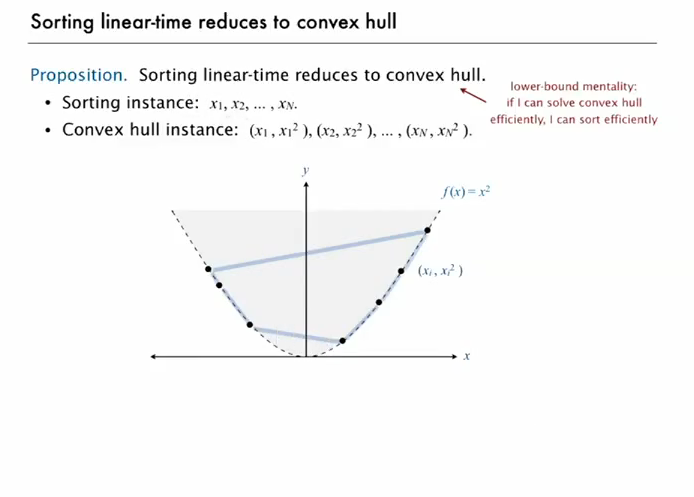 이미지를 잘 보면 convex hull 이
 y = x^2 선 위에 있다. 그리고 이 위에 있는 모든 점들이 정렬된 순서인걸 볼 수 있다. 그리고 정렬 대상이 2차원 좌표긴 하지만 quadratic decision tree model 내에 있으므로 정렬 문제로 linear-time reduction 이 가능하다.
Implication: Any ccw-based convex hull algorithm requires
Ω(N logN)ops (linear or quadratic tests)
이외에도
Element distinctness linear-time reduces to finding the mode because if the most frequent integer occurs more than once, then there is a duplicated integer.
Closest pair linear-time reduces to element distinctness because the distance between the closest pair is zero if and only if there is a duplicated integer.
두 원소가 같을때만 제거하므로, 위의 문제들로 linear-time reduction 이 가능하다.
Classifying Problems
두 문제 X, Y 가 복잡도가 같음을 보이고 싶다면
- show that
Xlinear-time reduces toY - show that
Ylinear-time reduces toX
그러면 X, Y 가 같은 복잡도를 가지고 있다고 말할 수 있다. 심지어 복잡도를 모름에도.
그리고 서로 reduction 이 가능하므로 한 문제에 대해 빠른 알고리즘을 개발해서, 다른 곳으로 적용이 가능하다.
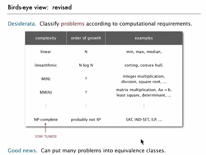
- use exact algorithm for tractable problems
- use heuristics for intractable problems
Reference
(1) Algorithms: Part 2 by Robert Sedgewick
(2) http://introcs.cs.princeton.edu
(3) xkcd image
(4) Convex hull image
(5) 전파거북이 - 좌표계 기반 벡터
(6) 소프트웨멤버십 - Convex hull
(7) Polar angle image
(8) sorting - convex hull image